More on Velocity Aliasing
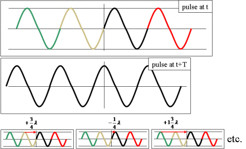
Although the samples of phase for consecutive pulses allow the determination of the Doppler shift, there is not a unique frequency which satisfies the observations. This is illustrated in Figure 5. All such solutions which satisfy the measured phases are known as aliases.
The phase shift measured by the radar is ambiguous to within multiples of 2π and consequently, the velocity calculated by the radar is
ambiguous to within multiples of
λ/2T meaning that the radar cannot distinguish between
velocity v
from
velocity v + (λ/2T) or..
-
or v + 2(λ/2T)
-
or v + 3(λ/2T) … etc
-
or v – (λ/2T)
-
or v – 2(λ/2T)
-
or v – 3(λ/2T) … etc
Figure 8: The phase shift of the radar pulse and corresponding ambiguity of the velocity
The radar simply assumes that the real phase shift is the one between
–π and +π and that the real velocity is the one between
-λ/4T and +λ/4T. Thus, Doppler radar only displays velocities between -VN and +VN
Atmospheric velocities outside this range will be misrepresented on the radar display – the real velocity will differ by a multiple of 2VN from the displayed value
This phenomenon is known as aliasing because the displayed velocity and the real velocity belong to a set of aliases that all look identical to the radar.
Velocity aliasing occurs because the mean radial motion of the target between radar pulses exceeds one half a wavelength and the resultant change in phase with time exceeds π/2.
The example below shows a velocity aliased PPI and RHI display. Note that the radar shows an alias of the actual echo as a result of the aliasing process.

Figure 9. Velocity and RHI display